Coin toss markov chains

1. The question

Let’s start with a simple question that will motivate the content of this blog. Not only is the answer beautiful, but it also helps us develop a framework for answering a whole family of such questions. The question goes like this - let’s say I have a fair coin (50-50 chance of heads and tails) and so do you. Both of us start tossing our coins. What is the probability that you will get three heads in a row before I get two heads in a row? It’s quite clear that I have a higher chance of winning (but don’t worry, my better odds are balanced by us obsessing over your victory throughout this post). Now, how do we go about calculating how much higher?

2. Thinking in terms of states

We can think of how close each player is to realizing his goal in terms of states. The first player (I) keeps tossing until he reaches two consecutive heads. So, we can define his state after n tosses as the number of consecutive heads he has so far. In the beginning, there are no tosses. So, the number of consecutive heads at that point is obviously zero.

If he gets a heads on the first toss then the number of consecutive heads after the first toss is one whereas if he gets a tails, it stays at zero. Hence, anytime a player is in the state “zero consecutive heads”, there is a 50% chance they will go to one consecutive head and 50% chance they will stay at zero consecutive heads after the next toss. The probability that the player will jump from zero consecutive heads to two consecutive heads in one toss is zero.

We can collect these three numbers into a vector of probabilities.

Similarly, if a player is at one consecutive head so far on any toss, the probability that they will be at two consecutive heads after the next toss is 50% and the probability of dropping back to zero is 50%. There will be a vector for transitions from this state as well.

So, each state has a vector of probabilities of going to each of the other states. We can collect these vectors and create a matrix.

This is what it will look like for me:

Note that the third row corresponds to the transitions from state 2. Since I plan on stopping once I reach two consecutive heads, I will not be making transitions to any other states once I reach state 2. That’s why state 2 (third row) has a probability 1 of simply transitioning to itself.

Similarly, you plan on stopping once you reach three consecutive heads. So, your transition matrix will look like this:

3. Probabilities at nth toss

Now, let’s think of the probabilities that I am in each of the possible states after a certain number of tosses. As said before, the probabilities at zero tosses are pretty clear. Both sequences are at zero consecutive heads. For the first sequence for example, there is a 100% chance I’m in state 0, a 0% chance I’m in state one (one consecutive head) and 0% chance I’m in state two. These three probabilities can be collected into a vector:

Now, what about after one toss. If I get a heads, I go to state one and stay in state zero if I get a tails. In other words, there is a 50-50 chance I’ll be in state 0 or state 1 after the first toss.

This argument might give you a feeling of deja-vu since we used the exact same one when constructing the matrix \(M_3\). In fact, we can get \(P_1\) by simply multiplying the \(P_0\) with \(M_3\).

Similarly to get \(P_2\), we multiply \(P_1\) with \(M_3\).

Which means that after 2 tosses, there is a .25 probability that I would reach my goal.

But from the previous equation we can say,

In general we can say,

Now, we can of course say this for any transition probability matrix \(M\) (non-negative entries and rows sum to one).

For your markov chain (you need three consecutive heads) we can similarly define the probabilities \(Q_n\), that you will be in each of the states 0, 1, 2 and your goal state of 3 consecutive heads. Like before,

\(Q_0\) is your state at zero tosses which is \((1,0,0,0)\) (with a probability of one, you are in state 0 - you haven’t tossed, so have obtained zero consecutive heads so far).

Let’s plot the probabilities that you will be in each of the states as a function of \(n\).

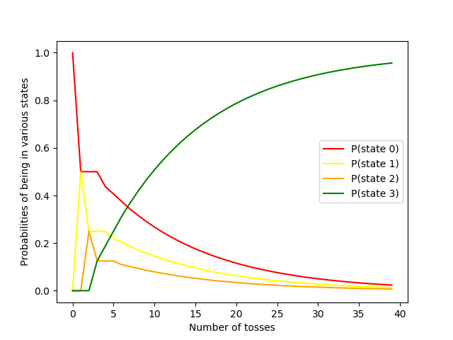
In the beginning, the starting state (0 consecutive heads) is obviously at 1.0. But it soon drops to zero. The other two non-absorbing states also make a climb initially since the final absorbing state must go through them. However, they quickly fall to zero as all the probability mass is sucked up by the absorbing state (in green).

Here is some simple, self-contained python code that shows how to calculate the probabilities of this sequence getting to the absorbing state as a function of the number of tosses (the green line in the plot).

import numpy as np

start = np.array([1,0,0])

# The transition matrix.
m_3 = np.matrix([
	 [.5,.5,0],
	 [.5,0,.5],
	 [0,0,1]
	 ])

## Probabilities of getting to absorbing state after n tosses.
# First raise the matrix to nth power
# then get the index of absorbing state
p_n = np.array([np.dot(start, np.linalg.matrix_power(m_3,n))\
						 [0,2]\
                               for n in range(100)])#Calculate this upto 100 tosses.

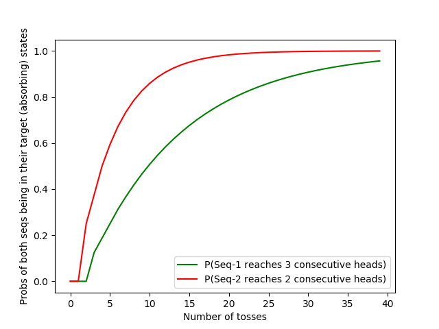
The plot will look very similar for the elements of the vector \(P_n\) of my states. However, my absorbing state (two consecutive heads) will be reached much quicker. In fact, let’s compare the probabilities me and you reach our goals (absorbing states: 2 heads and 3 heads respectively) by plotting them side-by-side.

4. Using the sequences to get the answer

All this is well and good but how is it going to help us get the number we’re looking for? What is the probability that you will reach three consecutive heads before I reach two? Let’s call this event \(A\). We then want to calculate \(P(A)\) (probability of event \(A\)).

Since we have the probabilities of both sequences being in each state, \(P_n\) and \(Q_n\), let’s try and use those. We can start with thinking of the event where we win in the nth toss. Let’s call this event \(A_n\). The only way \(A\) will happen is that one of the \(A_n\)s happen.

So, we can say that event \(A\) is the union of the events represented by \(A_n\).

Also, the \(A_n\)’s are mutually exclusive (meaning you can’t win on the third toss and the fourth toss). Because of this we can say:

So, if we get \(A_n\)’s, we can sum them to get the probability we are interested in.

What needs to happen for you to win on the nth toss?

1) The losing sequence (mine), given by \(P_n\) should not have reached it’s absorbing state by the nth toss. Otherwise, you didn’t reach three consecutive heads before I reached two. The probability is \((1-P_n[2])\).

2) The winning sequence (yours), given by \(Q_n\) should have reached a state where it needs just one more heads to win in the toss one earlier than the current toss. In this case, it means I should have reached two consecutive heads by the \((n-1)\)th toss. The probability is \(Q_{n-1}[2]\).

3) And finally, you should get a heads in the \(n\)th toss and complete the coup-de-grace. The probability of this is \(\frac{1}{2}\) since the coins are fair.

Combining those three events, we get -

And so we get to the most important equation of this blog,

There are other ways to represent the equation above. Here, we considered that the probability of you winning on the \(n\)th toss should be: \(\frac {Q_{n-1}[2]} {2}\). Taking it another way, we know that the probability that you will reach your goal on or before the \(n\)th toss is \(Q_{n}[3]\). Also, the probability that you will reach your goal on the \(n\)th toss is the probability that you reach it on or before the \(n\)th toss subtracted by the probability that you reach it strictly before the \(n\)th toss, which is just \(Q_{n}[3] - Q_{n-1}[3]\).

This means that equation (3) above can also be written as:

We can get \(P_n\) and \(Q_n\) by using equations (1) and (2) and simply multiplying the transition matrices \(n\) times. Of course, the sum in equation (3) goes to infinite terms and we can’t multiply the matrices infinite times. However, note that (as we can see from figure 1), \((1-P_n[2])\) will tend to zero as \(n\) becomes large (as the absorbing state - which is 2 - sucks up all the probability mass as \(n\) increases and this means one minus it’s probability tends to zero) and \(Q_{n-1}[2]\) will tend to zero for the same reason. So, the contributions to the sum of terms corresponding to large \(n\) become smaller and smaller. Hence, we can get a very, very good approximation by simply ignoring all terms associated with \(n\)s larger than some reasonable value (like 100 or 50).

Here is some python code that demonstrates this.

import numpy as np
start1 = np.array([1,0,0])
m_3 = np.matrix([[.5,.5,0], [.5,0,.5], [0,0,1]])

start2 = np.array([1,0,0,0])
m_4 = np.matrix([[.5,.5,0,0], [.5,0,.5,0],[.5,0,0,.5], [0,0,0,1]])

# p_n must always be one toss ahead of q_n_minus_1. So, when p_n is at toss 1, q_n_minus_1 
# should be at 0. When it is at 2, q_n_minus_1 should be at 1 and so on.
# that is why p_n starts with 1 and goes to 100 while q_n_minus_1 starts with 0 and goes to 99.
p_n = np.array([np.dot(start1, np.linalg.matrix_power(m_3,n))[0,2]\
                                     for n in range(1,101)])
q_n_minus_1 = np.array([np.dot(start2, np.linalg.matrix_power(m_4,n))[0,2]\
                                     for n in range(100)])

print("Prob(3 consec heads b4 2 consec heads):" + str(sum(q_n_minus_1*(1-p_n))/2))

Using this, we get that the probability we were after (you’ll get 3 consecitive heads before I get 2 consecutive heads) is 21.25%.

Similarly by flipping things, we can get the probability that I’ll get 2 consecutive heads before you get 3 consecutive heads

# Assumes you have run the previous block
p_n = np.array([np.dot(start2, np.linalg.matrix_power(m_4,n))[0,3] for n in range(1,101)])
q_n_minus_1 = np.array([np.dot(start1, np.linalg.matrix_power(m_3,n))[0,1] for n in range(100)])
print("Prob(2 consec heads b4 3 consec heads):" + str(sum(q_n_minus_1*(1-p_n))/2))

This shows that the probability that I will win is 73.98%.

Of course, the two numbers above don’t sum to one since there is also the third possibility of a draw (both reach their goals on the same toss).

We have now answered the question we posed at the starting of this blog. But often when one climbs to the top of a mountain, one simply sees more mountains on the other side. In that spirit, we will see what other questions we can answer with the tools developed in seeking the answer to this one in the next section (5).

Also, note that the approach of taking a large sequence formed by repeated matrix multiplication is somewhat ugly and inefficient. In section 6, we will improve on this and solve equation (3) in a cleaner, more efficient manner.

5. Other mountains

5.1. Even the odds

In the question we started the blog with, it was clear that the stakes were in my favor. Let’s consider now a contest where that isn’t obvious. I still need to get to two consecutive heads and you still need three. But to even the odds for you, your heads no longer need to be consecutive. As soon as you see three heads in total, you win.

This turns out to be a pretty close contest. Who should a gambler bet their money on?

We can solve this problem in a pretty similar manner to the previous one. Just construct the two Markov chains, use them to calculate the sequences of being in their various states after \(n\) tosses and plug the sequences into equation (3). &

My transition matrix will still be the \(M_3\) defined in section 2. Your transition matrix however, will not be the \(M_4\) defined there.

Now since you need three total heads, when you are in state \(i\), you don’t go back to zero if you get a tail on that toss. Instead, you simply stay at the state you were. In this way, I’m penalized more severely for a tails (I have to start over and you don’t).

Your new transition matrix, \(O_4\) will look like this:

And just like in section 4, we can solve this with the exact same code, just replacing your \(M_4\) matrix with \(O_4\) defined above.

import numpy as np
start1 = np.array([1,0,0])
m_3 = np.matrix([[.5,.5,0], [.5,0,.5], [0,0,1]])

start2 = np.array([1,0,0,0])
o_4 = np.matrix([[.5,.5,0,0], [0,.5,.5,0],[0,0,.5,.5], [0,0,0,1]])

# See previous code block in section 4 for detailed comments.
p_n = np.array([np.dot(start1, np.linalg.matrix_power(m_3,n))[0,2] for n in range(1,101)])
q_n_minus_1 = np.array([np.dot(start2, np.linalg.matrix_power(o_4,n))[0,2] for n in range(100)])

print("Prob(3 running heads b4 2 consec heads):" + str(sum(q_n_minus_1*(1-p_n))/2))

We see that the probability of you getting 3 running heads before my 2 consecutive is 36.74%. Your chances of winning have improved a little (from ~24% to ~37%), but there is more good news. When we flip things we get the probability that I will win:

# Assumes you have run the previous block
p_n = np.array([np.dot(start2, np.linalg.matrix_power(o_4,n))[0,3] for n in range(1,101)])
q_n_minus_1 = np.array([np.dot(start1, np.linalg.matrix_power(m_3,n))[0,1] for n in range(100)])
print("Prob(2 consec heads b4 3 running heads):" + str(sum(q_n_minus_1*(1-p_n))/2))

And this turns out to be 54.77%. So, my chances of winning have gone down from ~74% to ~55%. It seems there is a much higher chance the game will end in a draw (1-.55-.37 = 8%, up from 5% earlier).

So, your odds against me have gone from roughly 2:7 in the previous game to 2:3 in this one. That evens things out quite a bit, you’re probably still not happy, so let’s see what else we can do.

5.2. Unfair coins

In this section, we won’t settle for anything less than a completely even game. One way to do that is to go back to the old criterion (you need three consecutive heads while I need 2). However, we’ll let you cheat and use a biased coin (one that has a higher probability of heads than mine).

So, while my head still has a 50% chance of getting heads, yours will be higher. If your coin has a 100% chance of getting heads, note that your win is still not guaranteed. I could get heads on my first two tosses and that would mean you lose. The probability I’ll win is therefore 25% (\(.5 \times .5\) for the two heads I need).

The only way a draw can happen is if I get a tails on the first toss and then two consecutive heads. The probability of this is therefore 12.5% (\(.5\times .5 \times .5\)).

So, the probability that you’ll win is 1-.125-.25 = 62.5%.

But that tips things too much in your favor. We want the game to be even. Also note that if your probability of winning is 50%, you’re still going to be at an advantage because of the possibility of a draw, which will make my probability of winning less than 50%. We want to find the probability of heads \(p\) your coin should have for none of us to have an advantage.

For this, we just need to wrap the code from the blocks above in a function that takes the probability of heads as input (instead of hard coding to 0.5) and then we can a simple numeric method like bisection to find the \(p\) at which the probabilities of both of us winning are the same.

I simply plotted these probabilities with \(p\) in the code here. The result of which is:

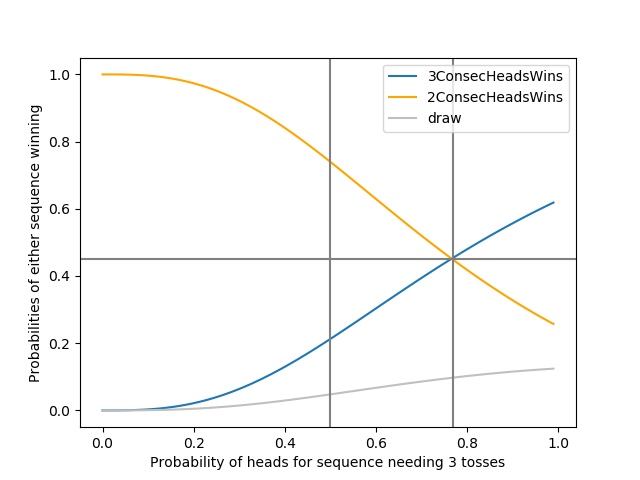
You can see from the plot that at \(p \sim 0.77\) at which point, both of us will have a \(\sim 45\%\) chance of winning.

5.3. Longer sequences

Now that we’ve evened the odds in the previous sub-section (just make your coin have a 77% instead of 50% chance of getting heads), we can try and test the power of these new wings we’ve developed. What if we go back to both of us having fair coins and wanted to get the probability that I reach 4 consecutive heads before you reached 3? What if it were me reaching 5 before you reaching 4? In other words, you still require one more consecutive head than me, but we’re gradually increasing the number of heads I need. In general, what is the chance I’ll reach \(n\) heads before you reach \((n+1)\) heads?

You can imagine now that the markov matrices become larger and larger as we increase \(n\) (there are \(n^2\) terms in the smaller one) and the chance that the game is resolved by the hundredth toss will become smaller and smaller (two or three consecutive heads would have appeared by the 100th toss, but ten consecutive heads is far less likely). So, we need to extend the sequences to a much larger number of tosses.

This makes the method we described earlier very slow. But, we can still use the faster method referenced earlier (will be described in section 6) to get the exact solution for \(n\) going all the way up to the late teens.

In any case, we plot the probabilities of me winning, you winning and a draw in the figure below. If you want to use the more efficient method described in section 6, you can do so with the aid of an open source library that goes along with this blog.

# To install the library, pip install stochproc from command line.
# hosted at - https://github.com/ryu577/stochproc
from stochproc.competitivecointoss.smallmarkov import *

ns = np.arange(2,15)
win_probs = []
for n in ns:
 	# The losing markov sequence of coin tosses that needs (n-1) heads.
 	lose_seq = MarkovSequence(get_consecutive_heads_mat(n))
 	# The winning markov sequence of coin tosses that needs n heads.
 	win_seq = MarkovSequence(get_consecutive_heads_mat(n+1))
 	# If you multiply the two sequence objects, you get the probability
 	# that the first one beats the second one.
	win_prob = win_seq*lose_seq
	win_probs.append(win_prob)

plt.plot(ns, win_probs)

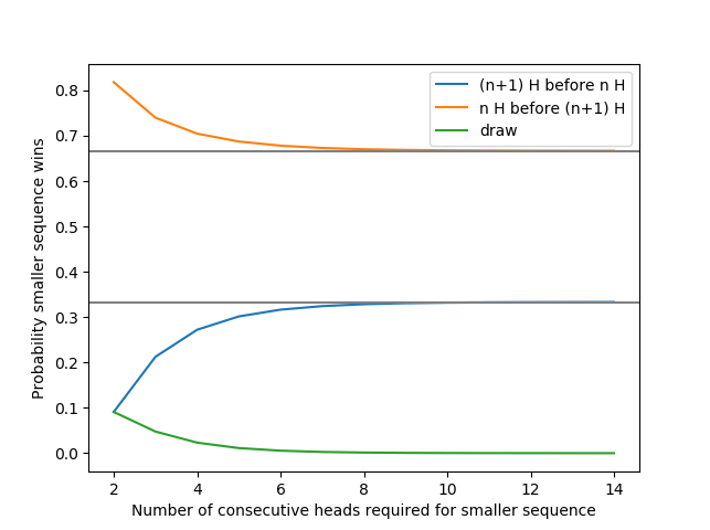
Looking at the figure, something surprising pops out.

As we increase the number of tosses I need, the probability of you winning starts approaching 33.33% or one third. Similarly, the probability of me winning starts approaching 66.67% or two thirds. It’s a little surprising that such simple numbers pop out.

And where there are simple numbers, there are elegant reasons.

Note that this game is like I have a coin that flips successfuly once in \(2^n\) (to get \(n\) heads in a row) and you have a coin that flips successfuly once in \(2^{n+1}\) and we ask who succeeds first.

What complicates matters is that I win ties. If \(n\) is large however, there will be very few ties.

Also if \(n\) is large, the chance of a run of \(n\) heads is very small, \(2^{-n}\). We can view each flip as a try by you to start a run of \(n+1\) heads, which happens with probability \(2^{-(n+1)}\) and a try by me to start a run of \(n\) heads, which happens with probability \(2^{-n}\).

Almost all attempts will fail for both of us. We can ignore those.

The chance that you win is then \(\frac {2^{-(n+1)}}{2^{-n}+2^{-(n+1)}}= \frac{\frac 12}{1+ \frac12} = \frac 13\).

The reason it starts lower when \(n\) is smaller is that we might both start succesful runs at the same time, at which point you win because your run finishes first. However for large values of \(n\), it becomes near impossible to succeed at the same time.

6. Closed forming the markov sequences

In the previous section, the approximation of cutting off at 100 tosses worked pretty well. This is because there is a very high chance the game would have ended well before 100 tosses (either one of the players reaching their goal).

What if however, we wanted the probability the first player gets 50 consecutive heads before the second one got 51. The probability that this would get resolved before 100 tosses is quite low, so cutting off at 100 would not give us a good approximation. And let’s say we needed to go to a million tosses to get a good approximation. Multiplying these large matrices millions of times would be a very computationally expensive affair to the point where we might not even be able to get the answer.

We can make this method more scalable to questions about large numbers of tosses and not dependent on multiplying matrices many times. But we’ll need some linear algebra - in particular, the concept of eigen decomposition - to do so.

To follow this section therefore, it is best you’re somewhat familiar with eigen value decomposition. It is basically a way to really x-ray matrices and see what they’re all about. The idea is that for the matrices \(M_3\) and \(M_4\), you can find three and four dimensional vectors respectively that when multiplied with them, don’t change. And then there are other vectors that are also special because they change, but are only scaled, not rotated.

If the matrix is \(n \times n\), you can find \(n\) such directions (including that one that wasn’t changed or was scaled by 1).

This translates to being able to write:

where the matrix \(E\) contains the special vectors that are scaled and not rotated as it’s columns.

Now if we look at equations (1) and (2), we basically need to raise the markov matrices to the power of \(n\), meaning multiply them with themselves over and over.

If we assume the matrix \(E\) from equation (4) is invertible, we can write (pre-multiplying both sides by \(E^{-1}\)).

Where

Now, if we want to square \(M_3\), we can use equation (5)

We can repeat this \(n\) times to conclude:

Since \(\Lambda\) is diagonal, we can write -

Now from equation (1),

If you multiply these out, this is equivalent to saying

Where \(C\) is a constant matrix of coefficients given by:

and \(E_{1,1}\), \(E_{1,2}\) and \(E_{1,3}\) are the elements of the first row of \(E\).

In equation (3), we only need \(P_n[2]\) which will be given by:

You can see here a proof that a stochastic matrix will always have eigen values less than one in magnitude. This means that the second and third terms of the expression above will tend to zero as \(n \to \infty\).

Since the sequence must eventually end up in the absorbing state for large enough \(n\) we must have,

Giving us,

Similarly, we will have a corresponding matrix \(D\) for your \(Q_n\) sequence and we can write:

Plugging (7) and (8) into equation (3) we get,

As long as we can construct the transition matrices for the two sequences of coin tosses and get their eigen values and eigen matrices, we can get the probability that one of them will beat the other using the approach above.

7. Other methods

I alluded earlier that once you climb a mountain, you’ll sometimes see other mountains on the other side. But there are probably multiple paths to the top of the mountain you currently on. And climbing via another paths is probably a unique experience in itself.

In this section, we’ll therefore consider some other methods to solve our original problem (what is the chance you get to three consecutive heads before I get to two consecutive heads?).

7.1. A “different” equation

There is a way to tame these processes coming from a completely different direction. By constructing a difference equation (see what I did there? Anyone? Anyone?). Ok, it might be too early for that pun if you haven’t heard of difference equations before.

Here is how this goes - consider my sequence of tosses where I’m aiming for two consecutive heads.

Let’s see if there is an alternate way to get the sequence of probabilities \(P_n\) used in equation (3). In particular, let \(a_n\) be the probability that I’ll reach my goal on the \(n\)th toss.

One thing we can say is that at the time when I reach my goal on the \(n\)th toss, the last two tosses I saw would have both been heads. Also, the third-from-final toss would have had to be a tails (otherwise, I would have won one toss earlier). The probability of this sequence of THH is \(\frac{1}{2}\times \frac{1}{2} \times \frac{1}{2} = \frac{1}{8}\).

Before these three tosses, my probability of winning would have been by definition, \(a_{n-3}\). But if I am to win in the \(n\)th toss, I need to exclude that event. And similarly \(a_{n-4}\) and so on. This means:

The second part of the equality follows since \(a_1 = 0\) (the probability of reaching two consecutive heads on the first toss is zero).

Now let’s define:

which represents the probability you would have won by the \(n\)th toss.

Plugging this equation into the previous one we get:

This is what I meant by “difference equation” it expresses a relationship for the difference of two consecutive terms of the series.

Simplifying further:

\begin{equation} b_n = b_{n-1} - \frac{1}{8} b_{n-3} + \frac{1}{8} \tag{9}\end{equation}

Now, we know \(b_n\) for the first few values of \(n\). When \(n=0\), there is no way I would be in my absorbing state of two consecutive tosses. Hence, \(b_0 = 0\). Even on the first toss, there is no chance I would have tosses two heads surely. So, \(b_1=0\) as well. When \(n=2\), there is a chance I would see two consecutive heads. For that, the first two tosses would have to both have been heads. The probability of this event is \(\frac{1}{2}\times\frac{1}{2} = 0.25\).

Now, we can use these and equation (9) to calculate the other terms of the sequence.

You get the idea by now, we can extend this as far as we like to get any \(b_n\). This is an alternate way to get the sequence we calculated in section 3 (\(P_n[2]\)) and used in section 4 to get the answer.

But, we still need to patiently iterate all the way to \(n\) starting from \(n=3\). This is similar to the way we were patiently multiplying matrices in section 3 to get the sequence of probabilities. However, we found a way in section 6 to replace the iterative method for calculating the probability sequence with a more elegant closed form. Is there a way we can find a closed form for this difference equation as well?

7.1.1. Closed form for the difference equation

The standard way to solve a difference equation like (9) is to separate into homogeneous and non-homogeneous parts, solve the homogeneous part using a polynomial guess and then make another guess for how the solution will need to be modified to make it compatible with the original, non-homogeneous equation.

First, let’s clean up equation (9) a bit:

\begin{equation}8b_{n}-8b_{n-1}+b_{n-3}=1\tag{10}\end{equation}

The homogeneous part of this equation is given by:

\begin{equation}8b_{n}-8b_{n-1}+b_{n-3}=0\tag{11}\end{equation}

Here, we make an educated guess (“ansatz” in German - we will make two of these guesses in this section which can make some people feel uneasy. If that is so, skip to the next sub-section (7.1.2) where we solve the same equation in a ‘more systematic’ manner).

We suspect the solution to this homogeneous equation might be:

Substituting this into equation (11), we get the characteristic polynomial:

The roots of which are given by \(l=\frac{1-\sqrt{5}}{4}, \frac{1+\sqrt{5}}{4}, \frac{1}{2}\)

Notice that the golden ratio, \(\phi\) is given by \(\phi = \frac{1+\sqrt 5}{2}\) which means we can express the roots of the characteristic polynomial of the homogeneous equation as:

Remeber we started off with the assumption that \(b_n'=l^n\). This means that the following will all work for \(b_n'\):

Meaning that any linear combination of these three solutions will also be a solution of equation (11). So in general,

\begin{equation}b_n’ = c_1 \left(\frac{\phi}{2}\right)^n + c_2 \left(\frac{1-\phi}{2}\right)^n + c_3 \left(\frac {1} {2}\right)^n\tag{12}\end{equation}

Now, how do we modify this solution of equation (11) above to get the solution of the original, non-homogeneous equation (equation (10))?

We know that \(b_n'\) satisfies equation (10) so we can write:

Let’s assume \(b_n' = b_n+c_0\)

So the equation above becomes:

To make this align with equation (10) we require \(c_0=-1\)

And this would mean \(b_n = b_n'-c_0 = b_n'+1\)

So, the general solution (\(b_n\)) of equation (10) can be written using this result and (12):

\begin{equation}b_n= c_1 \left(\frac{\phi}{2}\right)^n + c_2 \left(\frac{1-\phi}{2}\right)^n + c_3 \left(\frac {1} {2}\right)^n + 1\tag{13}\end{equation}

And for the two consecutive heads problem, we can use the first few values in the sequence \(b_n\) in particular, \(b_0=0\), \(b_1=0\), \(b_2=0.25\) and \(b_3=0.375\) to get the \(c_i\)’s. This is accomplished with the following python code:

import numpy as np
phi = 1.618033988749895
## The three roots
l1 = phi/2; l2 = (1-phi)/2; l3 = .5

mat = np.array([
            [1, 1,   1,    1],
            [1,l1,   l2,   l3],
            [1,l1**2,l2**2,l3**2],
            [1,l1**3,l2**3,l3**3]])

## The first four b_n's
bn = np.array([0,0,.25,.375])
cc = np.linalg.solve(mat,bn)
# cc is the vector of coefficients [c_0,c_1,c_2,c_3] = [1., -1.17082039, .170820393, 0]

7.1.2. Closed form for difference equation using matrix approach

If you were happy with the solution presented in 7.1.1, you can skip this one.

But some people feel like that qpproach requires a lot of guessing. How am I supposed to make all the right guesses after all? So, let’s explore another method to solve the difference equation which is based on the eigen values of a matrix just like the method in section 6 was.

To get a matrix, we need a system of equations while we have only one (eqn 9). To create a system of equations, let’s just add two more dummy equations.

Now, we can combine the above two equations with equation (9) and express this system in matrix form.

Now let \(\beta_n = \left(\begin{array}{c} b_n \\ b_{n-1}\\ b_{n-2}\\ \end{array} \right)\), \(\gamma = \left(\begin{array}{c} \frac{1}{8} \\ 0\\ 0\\ \end{array} \right)\) and \(M = \left( \begin{array}{ccc} 1 & 0 & -\frac{1}{8} & \\ 1 & 0 & 1\\ 0 & 1 & 0\\ \end{array} \right)\).

We then get:

And repeating this \((n-2)\) times we get,

Now, assuming \(M\) is diagonalizable (which it is) we can say:

And this would imply:

So we get:

\begin{equation}\beta_n = E\Lambda^{n-2}E^{-1}\beta_2 + E(I+\Lambda+\Lambda^2+\dots+\Lambda^{n-3})E^{-1}\gamma \tag{14}\end{equation}

Now, if \(\lambda_1\), \(\lambda_2\) and \(\lambda_3\) happen to be the eigen values of \(M\) then,

and,

meaning the \(\Lambda\) stays diagonal no matter how many times we multiply it with itself.

Remember, we are interested in the first element of \(\beta_n\) which is \(b_n\) and can be extracted by taking a dot product with a vector that has a 1 in the first position and zero at other positions.

Now, using the same arguments as in section 6, we can say that any component of the first term in the R.H.S of equation (14) can be written as:

Now to tackle the second term of equation (14). Observe that:

Here, we used the geometric series result:

Again, we see a similar pattern to the one utilized in equation (15) and so we can say:

meaning,

Adding equations (15) and (16), we get the first term in the L.H.S of equation (14), which is \(b_n\).

Now redefine: \(c_0 = d_0\), \(\frac{d_1+l_1}{\lambda_1^2} = c_1\) and so on we get:

Now, the eigen values of \(M\) are: \(\lambda_1, \lambda_2, \lambda_3 = \frac{\phi}{2}\), \(\frac{1-\phi}{2}\), \(\frac 1 2\), which are the same as the roots of the polynomial equation in the previous sub-section.

Substituting this into the previous equation we get equation (13) through this alternate linear algebra based route.

7.2. I’ll give you the answer on one condition

We started this blog with a simple to understand problem. The solution provided involved Markov chains and thinking in terms of states. That solution was like a silver bullet for a whole family of problems of this nature. In this section, we will pursue a simpler solution that involves just conditional probabilities.

Let’s define \(A\) as the event that you win.

Now, instead of thinking about the entire sequences of tosses, let’s think of just the very first toss for both sequences (the top one is yours and the bottom one is mine). Conditioning on these first two tosses we get,

Now, since all tosses are independent,

Which means that:

Now, if both of us get tails on our first tosses, that’s essentially the same as restarting the game. We might as well throw those tosses out and start from scratch since none of us is any closer to their goal.

Therefore its easy to see that:

Substituting into the previous equation we get:

Now let’s tackle the next term in order of difficulty, \(P\left(A| \begin{array}{c} T \\ H \end{array} \right)\). Let’s consider the various possibilities.

• If I get a tails on the next toss, the game is over and I’ve won. So, I have to get a tails on my second toss for you to win (or event \(A\) to occur). The probability of this is \(\frac 1 2\). The question becomes, what did you get on your second toss.
  • Now if you get a tails on the second toss (an event with probability \(\frac 1 2\)), the game would have been reset and the probability of you winning from there is \(P(A)\).
  • If you get a heads on your next toss, then we can throw away the first tosses. The probability you will win from here becomes \(P\left(A| \begin{array}{c} H \\ T \end{array} \right)\)

Putting all this together we get -

Next, let’s tackle \(P\left(A| \begin{array}{c} H \\ H \end{array} \right)\).

• If I get a heads on the second toss, the game is over since my first toss was already a heads. So, we don’t have to consider any possibility where that happens. So, our next two tosses can either be a heads for you and tails for me or tails for both of us.
  • If the our second tosses result in a heads for you and tails for me, the probability of this is \(\frac 1 4\).
    • If you then score a heads on the third toss as well (probability \(\frac 1 2\)), you win and it doesn’t matter what I got.
    • If you score a tails (probability \(\frac 1 2\)), things get more interesting.
      • If I score a heads (probability \(\frac 1 2\)), it’s effectively the same as me being on one heads and you being a one tails, which is \(P\left(A| \begin{array}{c} T \\ H \end{array} \right)\).
      • If I score a tails (probability \(\frac 1 2\)), then we both scored tails on our third tosses and any time that happens the game resets and the probability of you winning again becomes \(P(A)\).
  • If I get a tails on the second toss (probability \(\frac 1 2\)), it means we now both have tails and the game has reset. So the probability from here is \(P(A)\).

Putting all this together we have:

And using similar reasoning we can get:

Now, equations (17), (18), (19) and (20) are four equations in four unknowns and they can be solved to get \(P(A)\), which happens to be one of those unknowns.

7.3. One big chain

The original problem stated in this blog (you get three consecutive heads before I get two consecutive heads) was solved using Markov chains.

Is the fact then that there exists another method to solve this same problem, also relying completely on Markov chains, but having very little to do with the one discussed in section 4 a testement to the versetility and power of Markov chains?

Let’s go over this new method before we decide.

Here, instead of keeping track of the two coin toss sequences independently of each other, we define a single state for the whole game.

And this state is a collection of two numbers, the number of consecutive heads seen so far by you and me (first number, second number).

Before any of us tosses our coin, the state is of course \((0,0)\). After the first toss, if I get a heads and you get a tails, the state will be \((1,0)\); if both of us get heads, it will be \((1,1)\) and so on.

Also like the markov chains in the method described in section 4, we can’t let this one have an unbounded number of states. We need to stunt it’s state space by defining the ones that lead to a victory for either you or I as absorbing states. So for example, it will be impossible to get to state \((4,1)\) since you would have won and hence stopped as soon as you got three consecutive heads, hence never reaching four.

This makes \((3,0)\) and \((3,1)\) absorbing states that result in your victory while \((0,2)\), \((1,2)\), \((2,2)\) and even \((3,2)\) absorbing states resulting in my victory (you need to get 3 consecutive heads before I get two consecutive heads).

So, the possible states are (might as well express them in python code):

index2state=[(0,0),(1,0),(2,0),(0,1),(1,1),(2,1),(0,2),(1,2),(2,2),(3,0),(3,1),(3,2)]

Note that for the first six states, none of us has won. These are called transient states since they go to other states.

In the last six states, one of us has won and once the game reaches them, it stays in those states forever (since it concluded as soon as it reached them). Those states are called recurrent states.

Of the six recurrent states ((0,2),(1,2),(2,2),(3,0),(3,1) and (3,2)); (3,0) and (3,1) are the only ones where you win.

Now, the rules of the game obviously dictate some transition matrix between the states mentioned above.

• Any time the game is in state (i,j), if (i,j) is a transient state:
  • It will transition to (0,0) if both of us get heads (probability \(\frac 1 4\)).
  • It will transition to (i+1,0) if you get a heads but I get a tails (probability \(\frac 1 4\)).
  • It will transition to (j+1,0) if you get a tails and I get a heads (probability \(\frac 1 4\)).
  • It will transition to (i+1,j+1) if both of us get heads (probability \(\frac 1 4\)).
• Any time the game is in an absorbing state, it stays in the absorbing state with probability 1.

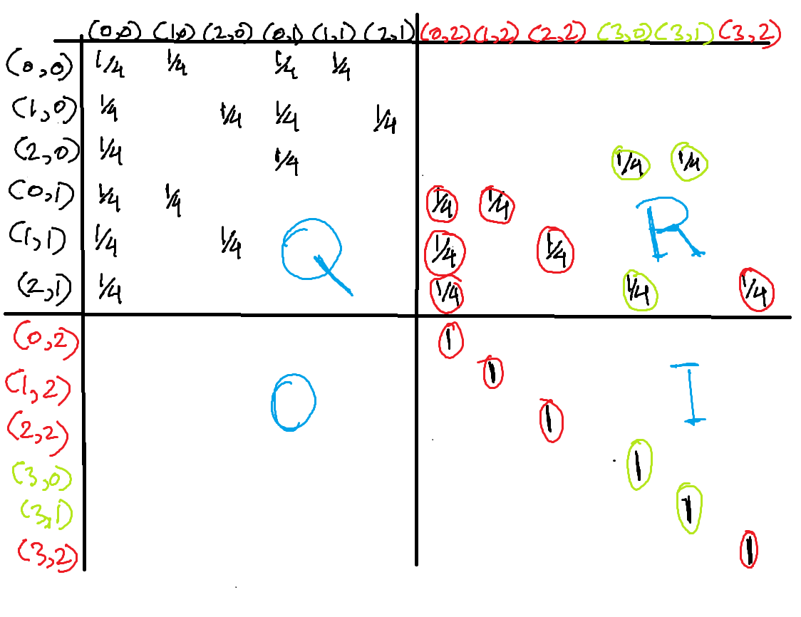
The matrix these rules correspond to is shown in the figure below. The transient states are represented in black, the absorbing states where you lose are represented in red and the ones where you win in green.

The larger matrix is divided into four sections. The top-left section is the sub-matrix for transitions between transient states. We call it \(Q\). The top-right is the sub-matrix for transitions from transient to recurring states. We call it \(R\). The bottom right is from recurring to recurring. Since recurring states stay in the same state and don’t transition anywhere else, this is simply an identity matrix.

Now, if we can find the probabilities that the game ends in each of the recurring states, we can use those to find the probability you’ll win since the recurring states corresponding to your victory are (3,0) and (3,1).

Given that we start in transient state \(i\), the probabilities that the game ends up in each of the absorbing states is given by the \(i\)th row of the matrix given by:

To see the reason, conditionin the absorption process from state \(i\) to state \(j\) based on what happens in the first transition: either the absorption happens in the first transition with probability \(R_{ij}\), or a transition occurs into some other transient state \(k\) with probability \(Q_{ik}\) and from there transitions until eventually absorbed with probability \(u_{kj}\). This can be expressed as the matrix equation

where solving for \(u\) generates the original equation above.

Here is some python code that generates the transition matrix \(M\) shown in the figure above, splits it into \(Q\) and \(R\) and then uses them to obtain \(U\) as per equation (21).

import numpy as np
m = np.zeros((12,12))
state2index = {(0,0):0,(1,0):1,(2,0):2,(0,1):3,(1,1):4,(2,1):5,(0,2):6,(1,2):7,(2,2):8,(3,0):9,(3,1):10,(3,2):11}
index2state = [(0,0),(1,0),(2,0),(0,1),(1,1),(2,1),(0,2),(1,2),(2,2),(3,0),(3,1),(3,2)]
for i in range(6):
    m[i,0] = 0.25
    m[i, state2index[(index2state[i][0]+1,0)]] = 0.25
    m[i, state2index[(0,index2state[i][1]+1)]] = 0.25
    m[i, state2index[(index2state[i][0]+1,index2state[i][1]+1)]] = 0.25
m[6:,6:] = np.eye(6)

q = m[:6,:6]
r = m[:6,6:]
u = np.linalg.solve(np.eye(6)-q, r)
print("Probability you win:" + str(u[0,3]+u[0,4]))