Optimum waiting thresholds

1. Optimum waiting threshold problem

Say it takes ten minutes for you to walk to work. However, there is a bus that also takes you right from your house to work. As an added bonus, the bus has internet, so you can start working while on it. The catch is that you don’t know how long it will take for the bus to arrive.

Now, being the productive person you are, you want to minimize the time you spend being in a state where you can’t work (walking to work or waiting for the bus).

If we knew exactly how long the bus was going to take on any day, this would be quite easy. If the bus is more than ten minutes away, simply start walking.

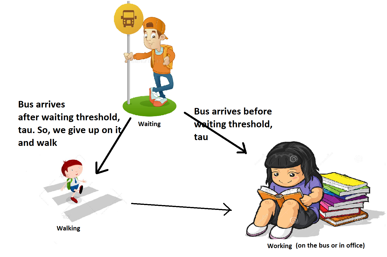
However, we know that real life is rarely so predictable. We probably have some distribution in mind for how much longer it will take for the bus to arrive, but not the exact time. Assume we have this distribution and it doesn’t change from one day to the next. Our strategy is simple - wait a certain amount of time for the bus (say 5 minutes) and if the bus doesn’t arrive by then, give up waiting and simply walk to work.

Now, assume that in parallel universes, you and your clones pick different wait-times. In one version, your clone always waits one minute, in another one, two minutes and so on.

How can you ensure that the total time you’ll spend waiting for the bus over a long period (say, a year) will be less than all the clones. In other word, what wait time should you pick so that the total time you spend either walking or waiting is minimized?

This clearly depends on the distribution for how long the bus is going to take. If we know this distribution, what can we do next?

2. Parametric survival models

Let’s say the time it’s going to take for the bus to arrive is \(T\), which is a random variable. Also, if we give up on the bus and decide to walk, the time it’s going to take is \(y\).

\[E[DT] = P(T \leq \tau). E [T|T<\tau] + P(T>\tau). (\tau + y)\]

Where :

• \(T\) is the organic distribution for the bus to arrive.
• \(\tau\) is the threshold for the time we will wait before starting to walk to the office.
• \(y\) is the time it will take for you to get to the office once we start walking.
• \(DT\) is the time we spend not working given waiting threshold, \(\tau\). It is a random variable that depends on \(T\) and \(\tau\).

As we can see, the equation above can be described as a simple expectation of two possibilities. Either the the bus will arrive before the threshold, \(\tau\) or, it won’t and we will walk to work losing a total time of \((\tau + y)\) (since we waited \(\tau\) before starting to walk and then spend \(y\) time walking). Now, to find the optimal value of \(\tau\) (which will minimize the L.H.S of equation (1)), we can differentiate equation (1) with respect to \(\tau\) and set it to zero. This leads us to the following condition (see appendix for how this comes about):

\begin{equation} \Rightarrow \frac{f_T(\tau)}{P(T\geq \tau)} = \frac{1}{y}\end{equation}

The expression in equation (1) has a very intuitive meaning. The expression on the L.H.S is called the “Hazard rate” of distributions describing the arrival times of certain events. The events being modelled are generally negative in nature (like defaults) hence the “hazard” in the name.

In our case though, the event we are anticipating is positive (the bus arriving - not so hazardous). It is the rate at which evens that the distribution is describing arrive.

Here, the rate is described as the inverse of the average time until the next event arrives as seen from the current state, instantaneously. Note that for most distributions, this rate itself will change with time so the average time until the next event won’t actually be the inverse of the instantaneous rate just as the instantaneous velocity of an accelerating object at a certain time can’t on its own predict the time the object will reach a certain point. The R.H.S is the inverse of the (deterministic) time it’ll take for you to get to work once we start walking. It too is then a kind of rate. It is when the rates corresponding to the two competing processes align that the optimal \(\tau\) is acheived.

In a nutshell, this points to the strategy - “at any point in time, go with the option that gives you a higher hazard rate”.

Now, how do we get the distribution, \(T\)? We can just observe how long the bus takes each and every day and then use the data to fit a distribution. This can be done using maximum likelihood estimation. In this context though, there is a bit of a wrinkle. And this is discussed next.

2.1 Dealing with censored data

So, we record the time it takes each day for the bus to arrive and fit a distribution to these observations. Simple, right? Well, not quite. The problem is, you probably can’t wait beyond a certain point for the bus. So, what about the times you waited say seven minutes, gave up and just walked to work? You know for sure that the bus took more than seven minutes. You just don’t know how much longer than seven minutes it took. What do you do with these observations? Should you simply throw them away? That would be a mistake since it would bias the data. The fitting method would never see values that are greater than the value at which they are getting censored, and wrongly assume those extreme values never occur in the real data.

To take these censored values into account, we need to modify the likelihood function. If there were no censoring, we might fit the distribution parameters to the data with a likelihood function that looks something like this:

\[L(\Theta; t_1, t_2, \dots t_n) = f_T(t_1, t_2, \dots t_n | \Theta) = \prod_{i=1}^n f_T(t_i | \Theta)\]

However, now we need to account for the censored data points as well. For this, we modify our likelihood function:

\[L(\Theta; t_1, t_2, \dots t_n, x_1, x_2, \dots x_m) = \left(\prod_{i=1}^n f_T(t_i | \Theta)\right) \left(\prod_{j=1}^m S(x_j|\Theta)\right)\]

Now, we can simply optimize this log likelihood function with respect to its parameters, calculate its hazard rate and use it in equation (1) to find the optimal wait threshold.

3. Alternate approaches

Apart from fitting the parametric distributions to the data and using equation (1), we can frame the problem in slightly different ways. In this section, we explore some of those ways.

3.1. Markov chain based approach

We can equivalently look at the process described above as a Markov chain. The two things we need for a Markov chain are states and the process that describes motion between the states. For example, we might define the states - “waiting for bus”, “walking to work” and “working”. We could then think of how we would move between these states.

In the Markov assumption, the probability of the state we will go to next only depends on the state we are in now. So, we can write these probabilities in the form of a matrix (source states along the rows and destination states along the columns).

\[\left( \begin{array}{ccc} P(T>\tau) & 0 & P(T<\tau) \\ 0 & 0 & 1 \\ 1 & 0 & 0 \end{array} \right)\]

We can also consider other aspects of the Markov chain. For example, instead of looking at the average time it takes to get to a new state, we can ask what proportion of time overall is spent on the road (walking or waiting for the bus).

Experiments show that for this simple Markov chain, the optimal threshold doesn’t change. We can see in the figure below that the threshold that minimizes the wait time to get from waiting to working (blue curve) is the same as the one that maximizes the proportion of time spent in a state where we can work (red curve).

However, in more complex markov chains with multiple thresholds, we might want to optimize this objective function.

3.2. Non-parametric approach

Let’s say we only wanted to evaluate thresholds that were less than the minimum censored value (say our current threshold is 10 minutes and so, all data points are censored at ten minutes and we’re sure we want to decrease it - so evaluate thresholds less than 10 minutes). Since we have complete information for all our data at the thresholds lower than 10 minutes that we wish to evaluate, we know exactly what would have happened if they were enforced. The figure below demonstrates this. Let’s say we want to move from the current threshold (in purple) to some lower threshold (in yellow). For the data points represented by the green dots, this is a good thing since they caused us to start walking anyway. We might as well have started walking earlier. For the orange points, it is less clear. If we walk

3.3. Hybrid approach

3.4. Piecewise hazard rates

Since equation (1) equates the hazard rates of two strategies, it is also possible to directly model them as a function of some covariates using the piecewise exponential model described in [1] and [2].

4. Experiments

In this section, we conduct a series of experiments where we start with a process such that we know the answer for the optimal threshold. We can then see how various models and approaches perform given just some data generated by this process. Each experiment is a set of answers to the following questions:

1. What process was used to generate the data? We have the following options:
   1. Lomax distribution.
   2. Weibull distribution.
   3. LogLogistic distribution.
   4. LogNormal distribution.
   5. Distribution given by an arbitrary hazard rate profile. As shown in equation (1), the hazard rate is a crucial element in defining where the optimal parameter will be. Also, the hazard rate can be used to get the PDF and CDF of the distribution. So, in theory we should be able to generate data from a distribution corresponding to an arbitrary function defining the hazard rate.
2. What is the process used to censor the data? We only consider censoring schemes where we don’t see data larger than the optimal threshold.
   1. None: No censoring at all.
   2. Deterministic censoring: All samples below the censor level are censored.
   3. Stochastic censoring: We randomly toss a coin and with probability p, censor the data point if it is eligible for censoring.
3. What model/methodology is being used to estimate the optimal wait threshold?
   1. We could use one of the distributions defined in question 1 and fit the data to them.
   2. We could use one of the non-parametric approaches.

If we exactly know the distribution generating the data, we have shown that we actually know the correct answer for the optimal waiting time by equation (2).

So, we can see which of our approaches comes the closest to this right answer.

4.1. Lomax data generation

In this section, we generate data from a Lomax distribution and see which models perform best at predicting the optimal threshold.

4.1.1. Deterministic censoring at value less than the optimal threshold.

First, let’s see how the Lomax distribution itself does.

Let’s start with the simple case where we have no censoring. Let’s generate some data from a Lomax distribution. Now, what happens when we apply the non-parametric methods we discussed to this data?

The results are best encapsulated in the figure below:

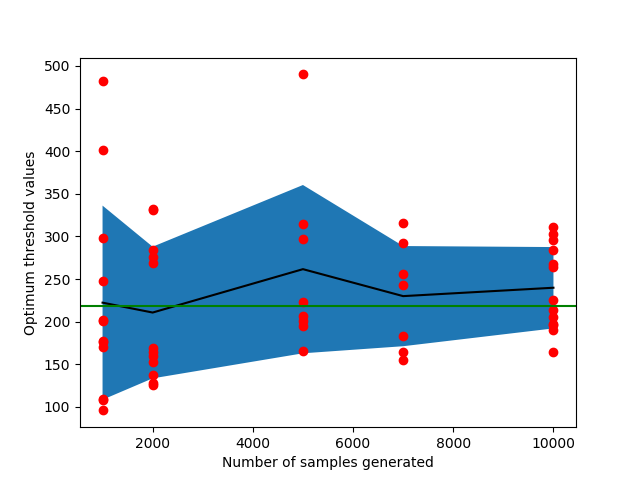
For the Weibull distribution, we get much higher optimal thresholds. For the LogLogistic distribution, we get slightly lower ones.

We should be careful to use a model that is capable of modelling the distribution we are after. If our assumption is incorrect, we can end up way off in terms of the optimal wait threshold.

4.1.2. Complete censoring

Here, we consider the case where we completely censor the data at some censor level. This process describes the scenario where we always wait exactly 10 minutes (say) for the bus and then start walking. How do our non-parametric approaches do in this scenario?

4.1.3. Random censoring

4.2. Non-standard processes

Our data might be generated by a process that doesn’t conform to any of the standard distributions.

5. Appendices

Now, \(E[T|T < \tau] = \frac{\int_0^\tau tf_T(t)dt}{P(T < \tau)}\)

\begin{equation}\Rightarrow E[T] = \int_0^\tau x f_X(x) dx + [1-P(X\leq\tau)] \times [\tau + Y] \end{equation}

To find the value of \(\tau\) that minimizes the expression in equation (1), we take the derivative with respect to it and set to zero.

\[\frac{dE[T]}{d\tau} = \tau f_T(\tau) - f_T(\tau) \times [\tau + Y] + [1-P(T\leq\tau)] = 0\] \[\Rightarrow 1 - P(T\leq \tau) = y f_T(\tau)\]

\begin{equation} \Rightarrow \frac{f_X(\tau)}{P(X\geq \tau)} = \frac{1}{Y}\end{equation}

7. References

[1] http://data.princeton.edu/wws509/notes/c7.pdf

[2] https://projecteuclid.org/download/pdf_1/euclid.aos/1176345693