Why is the gradient the direction of maximum ascent

This blog is based on a YouTube video explaining why the gradient is the direction of steepest ascent. Check it out.

I) Why bother?

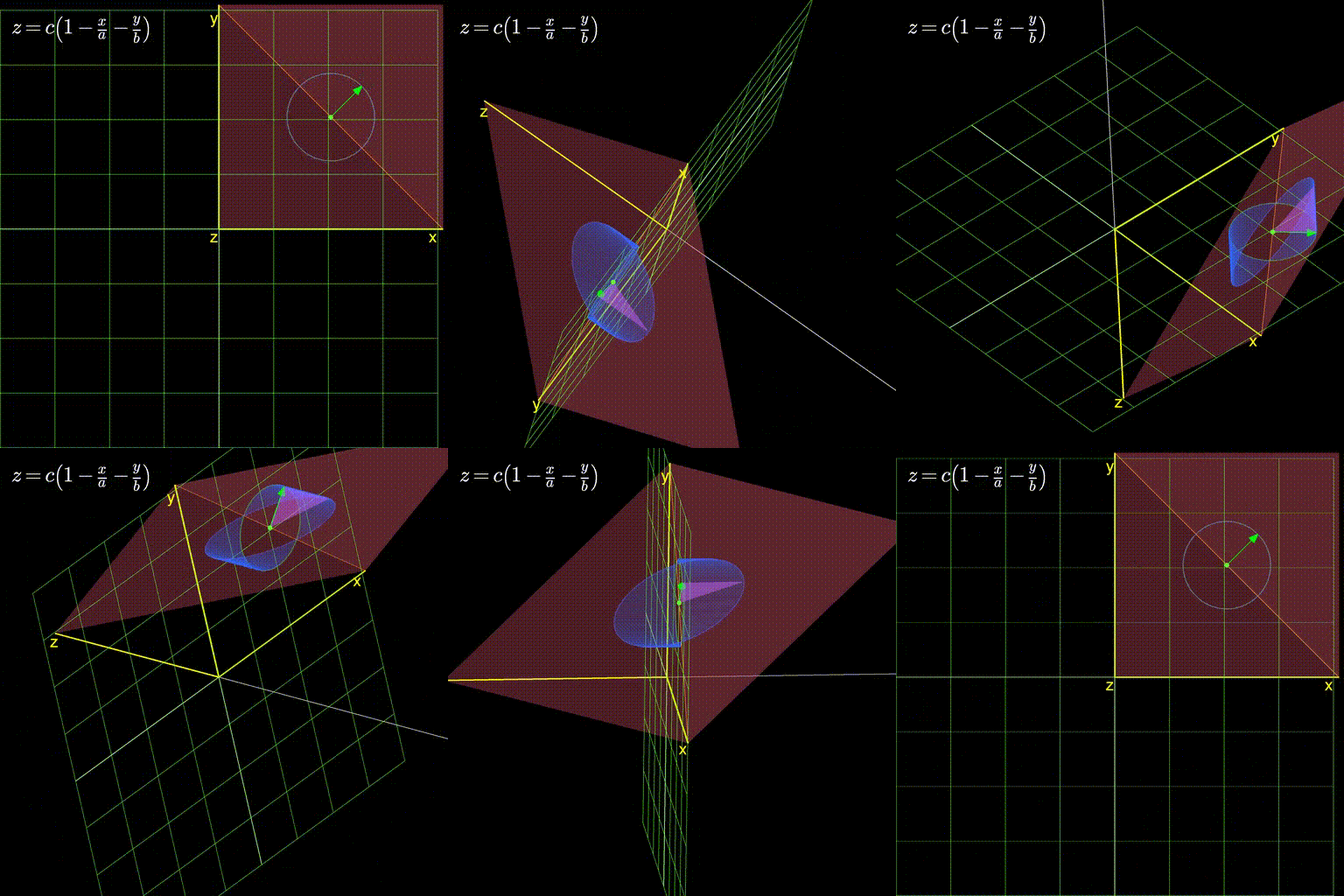
First, let’s get what might be the elephant in the room for some out of the way. Why should you read this blog? First, because it has awesome animations like figure 1 below. Don’t you want to know what’s going on in this picture?

Figure 1: A plane with its gradient

And second, because optimization is really, really important. I don’t care who you are, that should be true. I mean, it’s the science of finding the best. It let’s you choose your definition of “best” and then whatever that might be, tells you what you can do to achieve it. That simple.

Also, though optimization - being a whole science and all - has a lot of depth to it, it has this basic first order technique called “gradient descent” which is really simple to understand. And it turns out, this technique actually is the most widely used in practice. In machine learning at least, as the models get more and more complex, using complex optimization algorithms becomes harder and harder. So people just use gradient descent. In other words, learn gradient descent and you learn the simplest, but also most widely used technique in optimization. So, let’s understand this technique very intuitively.

II) Optimization brass tacks

As I mentioned in the last section, optimization is awesome. It involves taking a single number - for example, the amount of money in your bank account, or the number of bed bugs in your bed - and showing you how to make it the best it can be (if you’re like most people, high in the first case and low in the second). Let’s call this thing we’re trying to optimize \(z\).

And the implicit assumption here of course is that we can control the thing we want to optimize in some way. Let’s say it depends on some variable (say \(\vec{x}\)) which is in our control. So, at every value of \(\vec{x}\), there is some value of \(z\) (and we want to find the \(\vec{x}\) that makes \(z\) the best).

There is probably some equation that describes this graph. Say \(f(x,z) = 0\). But in the context of optimization, we need to express it in the form: \(z = f(x)\) (assuming the original equation is conducive to separating \(o\) from \(x\) in this way). Then, we can ask - “what value of \(x\) corresponds to the best \(z\)?”. If we have a nice continuous function, then one thing we can say for sure is that at this special \(x\), the derivative of \(z = f(x)\) (generally denoted by \(f'(x)\)) will be zero. Now if you don’t know what a derivative is (it’s the ratio of the amount \(o\) gets perturbed to the perturbation in \(x\), when we purposely perturb \(x\)) and why it should be zero when we achieve the best \(z\), I’d recommend checking out this video that covers this in detail.

III) What is a gradient

When the thing we are optimizing depends on more than one variable, the concept of the derivative extends to a gradient. So, if \(o\) from above depends on \(x\) and \(y\), we can collect them into a single vector \(\vec{u} = [x, y]\). So, with \(o = f(x,y) = f(\vec{u})\), the gradient of \(o\) becomes \(\Delta f(u) = [\frac{\partial f}{\partial x}, \frac{\partial f}{\partial y} ]\). And just like with the derivative, we can be sure that the value of \(\vec{u}\) that will optimize \(z\) will have both components of the gradient equaling zero.

As a side note, the gradient plays a star role in the Taylors series expansion of any smooth, differentiable function:

\begin{equation} f(\vec{u}) = f(\vec{a}) + (\vec{u}-\vec{a})^T \Delta f(\vec{a}) + \dots\end{equation}

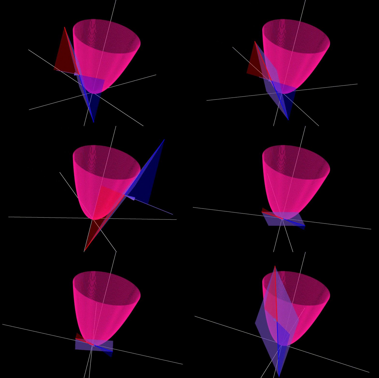
As you can see, the first two terms of the right side only involve \(u\), no squares, cubes or higher powers (those come up in the subsequent terms). Those first two terms also happen to be the best linear approximation of the function around \(u=a\). We show below what this linear approximation looks like for a simple paraboloid (\(z=x^2+y^2 = u^T u\)) at various points.

Figure 2: The best approximation of a paraboloid (pink) by a plane (purple) at various points

IV) Linear functions

We saw in the previous section that gradients are quite adequately represented with linear functions. So, we will restrict the discussion to linear functions going forward. For the equation of a linear function, we only need to know where it intersects the axes.

If we have just one dimension (the x-axis) and the intersection happens at \(x=a\), we can describe this by

\begin{equation}\frac{x}{a} = 1\end{equation}.

If we have two dimensions (x-axis and y-axis) and the line intersects the x-axis at \(x=a\) and the y-axis at \(y=b\), the equation becomes

\begin{equation}\frac{x}{a} + \frac{y}{b} = 1\end{equation}.

When \(y=0\), we get \(\frac{x}{a}=1\) which is the same as the equation above.

What if we have three dimensions? I think you know where this is going

\begin{equation}\frac{x}{a}+\frac{y}{b}+\frac{z}{c} = 1 \end{equation}

and so on (this by the way, is the red plane you saw in figure 1 above).

Now, we can see that all of the equations above are symmetric in \(x\), \(y\), \(z\) and so on. However, in the context of optimization one of them has special status. And that is the variable we are seeking to optimize. Let’s say this special variable is \(z\). In we want to express this as an optimization problem, we need to express the equation as \(z=f(x)\). If we do this to equation (4), what we get is

\begin{equation} z = c (1 - \frac{x}{a} - \frac{y}{b})\end{equation}

V) I want to increase my linear function. Where should I go?

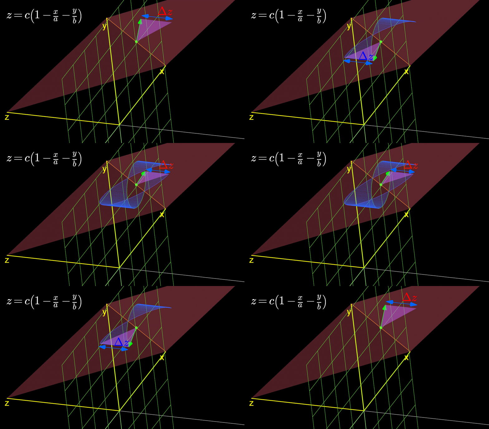
This is the central question for this blog. You have your linear function described by equation (5) above, with \(x\) and \(y\) are in your control. You find yourself at a certain value of \(x=x_0\) and \(y=y_0\). Let’s say for the sake of simplicity that \(z=0\) at this current point. You can take a step of 1 unit along any direction. The question becomes, in which direction should you take this step? This conundrum is expressed in figure 3 below showing the infinite directions you can possibly walk along. Each directions changes the objective function, \(z\) by a different amount. So, one of them will increase \(z\) the most while another will decrease \(z\) the most (depending on weather we want to maximize or minimize it).

Note that if we had just one variable in our control (say \(x\)), this would have been a lot easier. There would have been only two directions to choose from (increase \(x\) or decrease \(x\)). As soon as we get to two or more free variables however, the number of choices jumps from two to \(\infty\).

Figure 3: The infinite directions we can move along. Which one should we choose?

Now, we want to find the directions along which \(z\) changes the most. So let’s do the opposite (say, because we’re a little crazy?). Let’s look for the direction where \(z\) doesn’t change at all. If you look at the figure above carefully, you’ll see that this happens when the green arrow aligns with the orange line. And then if you continue staring, you might notice that the \(z\) changes the most when the green arrow is perpendicular to the orange line.

So, it seems like that orange line can provide some insight into this problem. What is the orange line then? Well, its clearly where our plane intersects the green grid representing the x-y plane (the grid along which we can move). And what would the equation of the x-y plane be? It would be \(z=0\). In other words, \(z\) does not change on it. So, since the orange line lies completely on the grid, it must also have \(z=0\) everywhere on it. No wonder \(z\) refuses to change when our green arrow causes us to simply move along the orange line.

As for the equation of the orange line, it is where the equations of the plane -

\[\frac{x}{a} + \frac{y}{b} + \frac{z}{c} = 1\]

and x-y grid; \(z=0\) are satisfied simultaneously. This gives us

\[\frac{x}{a} + \frac{y}{b} = 1\]

Now, it is clear from the equation of the orange line above that when \(y=0\), \(x=a\). So, the position vector of the point where it cuts the x-axis is \(\vec{o_x} : [a,0]\) (\(o\) for orange). Similarly, the point where it cuts the y-axis is \(\vec{o_y} : [0,b]\). Now that we have the position vectors of two points on the line, we subtract them to get a vector along the line (\(\vec{o}\)).

\begin{equation}\vec{o} = \vec{o_x} - \vec{o_y} = [a,0] - [0,b] = [a, -b]\end{equation}

Now, if we can show that the gradient is perpendicular to this vector, we are done. That will give us some intuition around why the gradient changes \(z\) the most.

VI) Gradient of the plane

Applying the definition of the gradient from section III to the equation of the plane (equation (5) above) we get -

\begin{equation} \frac{\partial z}{\partial x} = \frac{c}{a} \ , \frac{\partial z}{\partial y} = \frac{c}{b} \end{equation}

This makes the gradient:

\begin{equation} \Delta z : [\frac{c}{a}, \frac{c}{b}]\end{equation}

Now, we know that for two vectors to be orthogonal, their dot product must be zero. Taking the dot product or the gradient of the plane (from equation (7)) and the vector along the orange line (from equation (6)) we get,

\begin{equation} (\Delta z)^T \vec{o} = [\frac{c}{a}, \frac{c}{b}] [a, -b]^T = a.\frac{c}{a} - b.\frac{c}{b} = 0 \end{equation}

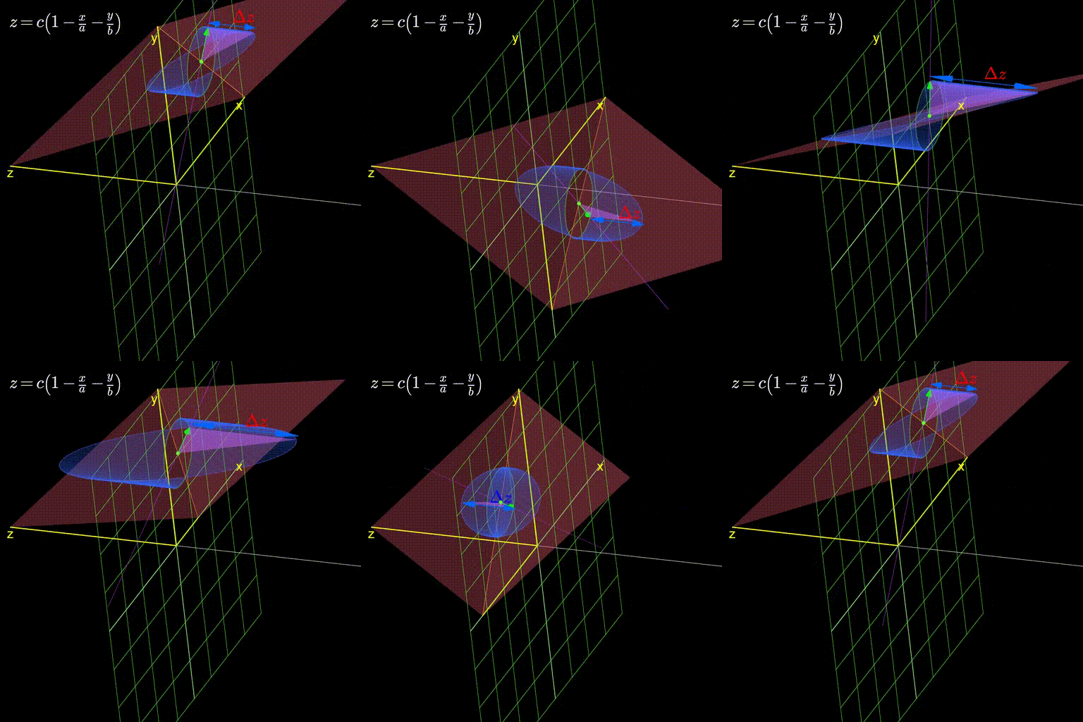
And there we have it, the gradient is aligned with the direction perpendicular to the orange line and so, it changes \(z\) the most. It turns out that going along the gradient increases \(z\) the most while going in the opposite direction to it (note that both these directions are orthogonal to the orange line) decreases \(z\) the most.

I’ll leave you with this visualization demonstrating how as we change the plane, the gradient continues to stubbornly point in the direction that changes it the most.

Figure 4: As we change the plane, the gradient always aligns itself with the direction that changes it the most