Solve a system of polynomial equations - Buchbergers algorithm for computing Groebner basis
What are polynomials?
First, let’s define very quickly some basic terms.
- Monomials are functions in one or more variables where we are only allowed multiplication and non-negative integer exponents. For example, \(x^2 y\) is a monomial in the variables \(x\) and \(y\).
- Polynomials are functions in one or more variables that involve the operations of addition, subtraction, multiplication and non-negative integer exponents. This means, they are basically sums of monomial terms. Here is an example of a polynomial in three variables, \(x, y, z\).
Linear Ideals
Before getting into polynomials, lets consider the simpler special case of linear equations (polynomials where the powers of the variables in each monomial sum to no more than one). Let’s say we are given a system of linear equations.
\begin{equation} a_{1,1} x + a_{1,2} y - b_1 = 0 \end{equation}
\begin{equation} a_{1,2} x + a_{2,2} y - b_2 = 0 \end{equation}
Now, we can apply any single variable functions, \(f_1(u)\), \(f_2(u)\) such that \(f_1(0) = 0\) and \(f_2(0) = 0\) to the two equations and the sum would still be an expression that equals \(0\).
\begin{equation} f_1(a_{1,1} x + a_{1,2} y - b_1 ) + f_2(a_{1,2} x + a_{2,2} y - b_2) = 0 \end{equation}
However, equations (1) and (2) are linear equations while this is not necessarily true for equation (3). The only functions \(f_1(u)\) and \(f_2(u)\) for which equation (3) is also a linear equation are of the form -
\begin{equation} f_i(u) = c_i u \end{equation}
Here, the \(c_i\) are constants, so these \(f_i\) are just linear equations that pass through the origin. The operations described above would be the famous row operations if the equations were written in matrix form.

Now, the set of all linear equations obtained through this process is infinite, but in general smaller than the set of all possible linear equations that exist. We call this smaller set the “Ideal” of linear equations. Given the two equations (1) and (2), we can generate every other linear equation in this Ideal. So, the two equations form a basis of this ideal. However, we could choose two other equations from the ideal and those would form a valid basis as well (say, the first one by adding equations (1) and (2) and the second by subtracting (2) from (1)). The natural question then becomes, which of these sets is the “best”? There is infact a basis which looks a lot more natural and elegant than all the others. And this is the Echelon form, where as far as possible, each equation involves only one variable (or as few variables as possible). This makes the region where all of these equations are solved simultaneously very obvious to see (if each equation involves just one variable, solving for that variable is trivial). We can acheive this special basis through Gaussian elimination, where we systematically perform row operations until each equation involves just one variable.
Polynomial Ideals
Polynomial bases are a generalization of systems of linear equations to polynomial equations. Let’s again consider a system of (two) quadratic equations in two variables.
\begin{equation}g_a(x, y) = a_{0,0} + a_{1,0} x + a_{0,1} y + a_{2,0} x^2 + a_{0,2} y^2 + a_{1, 1} xy = 0 \end{equation}
\begin{equation}g_b(x, y) = b_{0,0} + b_{1,0} x + b_{0,1} y + b_{2,0} x^2 + b_{0,2} y^2 + b_{1, 1} xy = 0 \end{equation}
Again, applying functions \(f_1\) and \(f_2\) to these eqations still results in a valid expression but that expression is not necessarily a polynomial equation. So, what should the functions be to ensure that the resulting equation is also a polynomial?
Unlike linear equations (where multiplying two of them produces a quadratic, not necessarily linear equation), if we multiply two polynomial equations, we just get another polynomial equation. So, we can multpily both equations (4) and (5) by any other polynomials in the same variables (\(x\) and \(y\)) and still end up with polynomials. We can then add these new polynomials together and get yet another polynomial. In other words, can consider \(f_i(u) = c_i u\) where now, \(c_i\) is a polynomial in all the variables that \(g_a\) and \(g_b\) are are polynomials in (here \(x\) and \(y\)). Then, we get -
\begin{equation} g_a(x,y) c_a(x,y) + g_b(x,y) c_b(x,y) = 0\end{equation}
For different polynomial functions, \(c_a\) and \(c_b\), we will end up with different polynomial equations. These will again (just like with linear equations) form an infinite set which is probably smaller than the set of all possible polynomial equations in \(x\) and \(y\). And since all we need to generate this set are \(g_a\) and \(g_b\), we can consider them a basis of this set. Just like linear equations, the set of these polynomial equations is called the “Ideal” of polynomial equations. And again, we can think of alternate bases for this ideal (other than (\(g_a\), \(g_b\))). Like the Echelon form for linear equations, can we think of a collection of polynomial equations where each of them has as few variables as possible. This will again make the task of finding points that satisfy them simultaneously very easy. For polynomial ideals, this special basis is called a “Groebner basis”. It is a fairly recent invention (1965).
Applications of Groebner Basis
It is beyond the scope of this blog to go into the details of how Groebner basis are calculated and what their properties are. For that, you can read the book on Ideals, Varieties and Algorithms by Cox, Little and O Shea (henceforth, “CLO”), which I highly encourage you to do (I personally completed the first two chapters at the time of writing). We can however, treat them like a magic black box that produces a special type of basis for polynomial ideals. A basis that makes all problems go away. And by doing so, we can solve a surprising array of very practical problems.
As you can imagine, systems of polynomial equations occur in all kinds of applications. And whenever they do, Buchbergers algorithm and Groebner basis is there to foil them.
This paper is an excellent resource on this. Here are some examples -
- Optimization problems where the objective function and constraints are polynomial equations. Minimizing sum of squared errors immediately comes to mind.
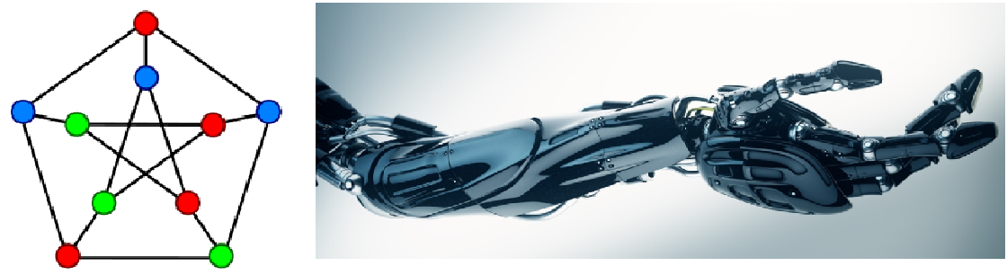
- Robotic motion planning - let’s imagine a robotic arm consisting of various limbs. We can imagine that the length of each limb will be fixed, so the range of motion it can perform in isolation will be restricted to a circle at the hinge. When we consider many such limbs and want to find the best way to reach for an object, we get a system of polynomial equations.
- Finding the minimum number of colors needed to paint a graph such that no adjacent vertices have the same color. This is called the chromatic number of the graph.
Implementation in C#
The algorithms provided in the CLO book were implemented in this git repo. While there are other implementations of Buchbergers algorithm on Github, I felt a new one was needed since -
- None of them were in C#.
- None of them were well commented and designed to be easily understandable. So, I took care to comment this code really well and since it follows the most popular book on this topic very closely, it is a very good companion for someone reading through it.
In the code, you will find C# classes for most of the algebric objects discussed in the previous sections and methods implementing the algorithms from the book. The various classes that are a part of this solution form a hierarchical structure:
PolynomialBasis
│
└───Polynomial
    │
    └───Monomial
What this means is that a collection of monomials form a polynomial and a collection of polynomials form a polynomial basis. Since a polynomial basis is simply a set of polynomials, I used a HashSet to store the polynomials. However, when we think of monomials in a polynomial, the order matters. Also, we need to store not just the monomials but also their coefficients. So, I used a SortedDictionary of monomials to back up the polynomial object.
The code starts with the building blocks like LCM (Least Common Multiple), polynomial division, etc. and builds up to Groebner basis. Some applications of Groebner basis are also provided. You can execute the code via Program.cs. In the comments and documentation for the code, “CLO” referes to the CLO book
Let’s see an example of how to use this code to solve systems of polynomial equations.
A new Polynomial basis object can be instantiated through strings which contain polynomial equations in human readable form -
And then, the Buchbergers algorithm can be called to simplify the basis to a more natural Groebner basis. Then, we use the pretty print function to show this new basis.
This will produce output in the following format -
Polynomial - 0
 + 0.67-0.78 z - 0.22 z^2 - 0.11 z^3 +  x

Polynomial - 1
-2.67 - 0.22 z + 0.22 z^2 + 0.11 z^3 +  y

Polynomial - 2
-18 - 12z + 13z^2 + 5z^3 +  z^4
Notice that the last polynomial involves only \(z\). We can use it to find possible solutions for this variable. The second to last one then, contains only \(z\) and \(y\). So, the values of \(z\) calculated from the previous equation can be substituted to get possible values of \(y\). Similarly, the first equation can be used to calculate \(x\).
Now, let’s peer at the machinery behind this. Here is the simplest (and most inefficient) version of Buchbergers algorithm as provided in section 2.7, Theorem 2 for computing the Groebner basis (\(g_1, g_2, \dots , g_t\)) of a polynomial ideal, starting with an arbitrary basis (\(f_1, f_2, \dots , f_s\)). Don’t peer at it too closely here before reading the background in the book. This is meant as an illustration of how the algorithms in the book translate to the C# code. Note that the more efficient version of the Buchbergers algorithm given in theorem 11 in section 2.9 is also implemented.
| INPUT: \(F = (f_1,f_2, \dots , f_s)\) | |
| OUTPUT: A Groebner basis \(G = (g_1, \dots , g_t )\) for \(I\), with \(F \subset G\) | |
| \(G := F\) | |
| REPEAT | |
| \(G' = G\) | |
| FOR EACH PAIR \(\{p ,q\}\), \(p \neq q\) in \(G'\) DO | |
| \(S := \overline{S(p, q)} ^ {G'}\) | |
| IF \(S \neq 0\) THEN \(G := G \cup {S}\) | |
| UNTIL \(G = G'\) |
And here it is implemented in C# (from the PolynomialBasis.cs file from the repo):